M7-Quantitative Decision Methods-S2 - Probability

The basic relationships of probability are: {{{ P(A or B) = P(A) + P(B) // for mutually exclusive events P(A or B) = P(A) + P(B) - P(A and B) // for non-mutually exclusive events P(A and B) = P(A)*P(B) for independent events P(A and B) = P(A)*P(A or B) for dependent events }}}

Binomial distribution The binomial distribution is used where there are two outcomes and the probability of an outcome remains constant regardless of the # times the experiment is repeated (Independent events: $P(r)={n \choose r}p^{r}(1-p)^{n-r}$

An elementary example is this: roll a standard die ten times and count the number of sixes. The distribution of this random number is a binomial distribution with n = 10 and p = 1/6. As another example, flip a coin three times and count the number of heads. The distribution of this random number is a binomial distribution with n = 3 and p = 1/2.

Try out a bit with /static/files/MBI/Module%207/binomial.xlsx

Part of M7-Quantitative Decision Methods-S2 - Probability distributions See also:http://en.wikipedia.org/wiki/Binomial_distribution Basic relationships in probability

• Mutually exclusive events
• Non-mutually exclusive events
• Independent events
• Dependent events

If events A and B are mutually exclusive then: {{{ P(A or B) = P(A) + P(B) }}}

If events A and B are non mutually exclusive then: {{{ P(A or B) = P(A) + P(B) - P(A and B) }}}

If events A and B are independent then: {{{ P(A and B) = P(A) X P(B) }}}

If events A and B are dependent then:

A)

Where P(B | A) is the probability that B occurs given that A already happened.

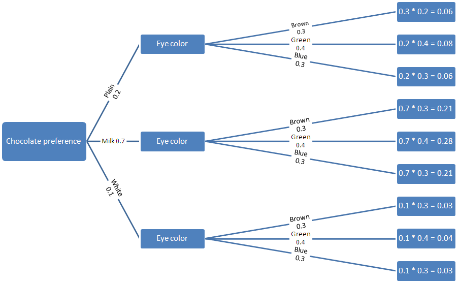
Part of M7-Quantitative Decision Methods-S2 - Probability and decision trees Probability tree For Independent events it is simple multiplication of each choice: {{{ P(plain chocolate) * P(brown eyes) = 0.2 X 0.3 = 0.06 }}}

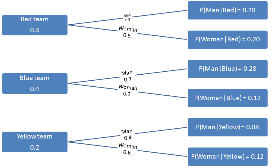
For Dependent events it is using conditional probability. Red) + P(Woman

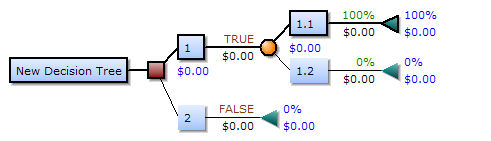
Part of M7-Quantitative Decision Methods-S2 - Probability and decision trees Expected value The expected value of an outcome converges to the long term average result of the probability of an outcome multiplied by the probability of an outcome: $E(x)=\sum (x*P(x))$ Decision Trees Decision support tool that uses a tree-like graph or model of decisions and their possible consequences, including chance event outcomes, resource costs, and utility. A decision tree combines the idea of a Probability tree with Expected value.

A decision tree consists of 3 types of nodes: 1. Decision nodes - commonly represented by squares 2. Chance nodes - represented by circles 3. End nodes - represented by triangles

Source: http://en.wikipedia.org/wiki/Decision_tree Bayes Theorem Bayes Theorem proposes to look at the end of a sequence of events, so we know the outcome, and we wish to find the probability of a certain event in the sequence (posterior probability). As an example say a production line has 3 machines A, B and C.

A	B	C
40%	50%	10%

If we see defective items it is not certain from which machine they came. With Bayes theorem it is possible to identify the most likely machine and check that one first. Suppose the waste rates are:

A	B	C
6%	1%	10%

Then the probabilities per machine are:

• A 0.4
  • 0.94 acceptable: 0.376
  • 0.06 defective: 0.024
• B 0.5
  • 0.99 acceptable: 0.495
  • 0.01 defective: 0.005
• C 0.1
  • 0.90 acceptable: 0.090
  • 0.10 defective: 0.010

The overall probability of a defective item is: {{{ P(defective) = 0.024 + 0.005 + 0.010 = 0.039 }}} This can also be written as A or B or C)

To look at a particular outcome, for example for Machine A and a defective item, we could write the probability as {{{ P(A and defective) = P(defective/defective from any machine) }}} Which is: {{{ P(A and defective) = P(0.024 / 0.039) = 0.615 }}}

The general formulation of Bayes Theorem is: Failed to parse (syntax error): {\displaystyle {P(A_i|X)} =\frac} {{P}(X|A_i) P(A_i)}{\sum_{i=1}^{i=n}{P(X | A_i) P(A_i)}}

Applied to the example $P(X|A_{i})$ represents the percentage of production that goes to machine $A_{i}$. $P(A_{i})$ represent the chance that this machine delivers a defective item. The multiplication of the two represent the overall probability that a specific machine delivered a defective item. ${\sum _{i=1}^{i=n}{P(X|A_{i})P(A_{i})}}$ represents the total overal chance of getting a defective item in the full population (0.024 + 0.005 + 0.010 = 0.039)

Part of: M7-Quantitative Decision Methods-S2 - Probability and decision trees See also: http://en.wikipedia.org/wiki/Bayes%27_theorem